
HSC Viewer menu bar
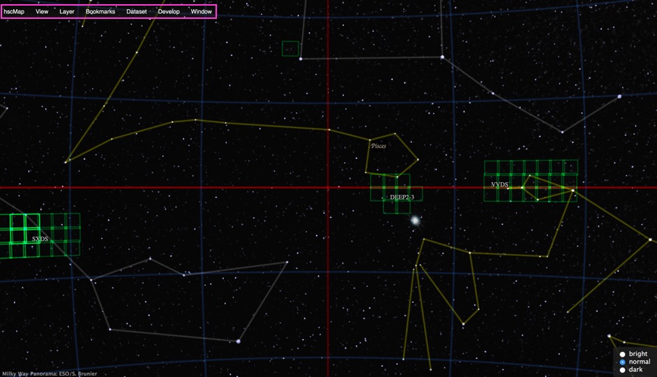
Fig. 1 The menu bar is located in the pink box in the upper left of the screen.
hscMap
- About hscMap: A version can be seen.
- Preferences: (Another window will open.)
- Wheel Sensitivity: Please adjust using the bar.
- Mouse
- Intertia: You can adjust the deceleration of your mouse.
- Mouse Response: You can adjust the sensitivity of the mouse.
- WebGL: If your PC runs slowly while using the HSC Viewer, try reducing the resolution.
- Max Canvas Size: Please enter the maximum pixel number.
- Retina: high resolution support
View
- Gnomonic Projection: Display using gnomonic projection
- tereographic Projection: Display using stereographic projection
- Celestial Globe: Display the celestial globe
- Zoom: Set the step size for Zoom In and Zoom Out
- Go to the Coordinate: Go to the position designated in the coordinates window
- North Up: set North to the top of the screen
- Diurnal Motion: apply diurnal motion
- Speed: set the speed of diurnal motion with the bar
- Fullscreen: make the window full-screen
-
Select from 90° to 1 arcminute (1/60°). With "Zoom In" and "Zoom Out", you can also enlarge or reduce the image size smoothly.
-
Please enter the right ascension (RA) and declination (Dec) of where you want to go.
(Example1) RA=150.0903°, Dec=+2.2103° is entered as "150.0903 2.2103"
(Example2) RA=10h 00m 21.67s, Dec=+2° 12′ 37.19″ is entered as "10:00:21.67 +02:12:37.19"
Layer: detail settings
- Gird: display grids
- Hipparcos Catalog: display foreground stars listed in the Hipparcos Catalog
- Constellations: display constellation lines
- Constellation Names: display constellation names
- Tract Frames: display tract frames in green
- Field Names: display observation field names such as DEEP2-3 or VVDS
- Background
- Show: display the background
- The Milky Way panorama (ESO): select the Milky Way taken by S. Brunier at the European Southern Observatory (ESO) as the background
- National Astronomical Observatory of Japan, Mitaka Campus: Select the NAOJ Mitaka Campus athletics field with the 50-cm Telescope for Public Outreach as the background
- Gravitational Waves
- Contour: Display the probability contour for the location of the gravitational wave source is located (the central area was the most probable).
- See Fig. 1 of the "How to operate the HSC Viewer" page for more information about tracts.
Background Display
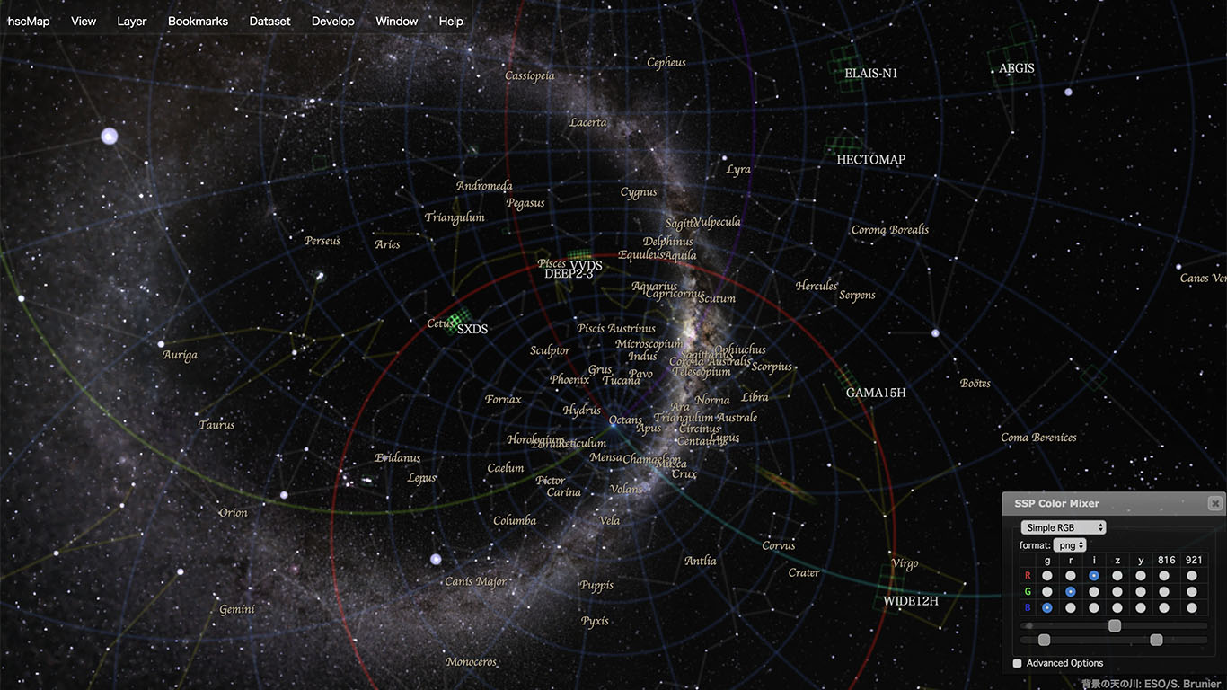
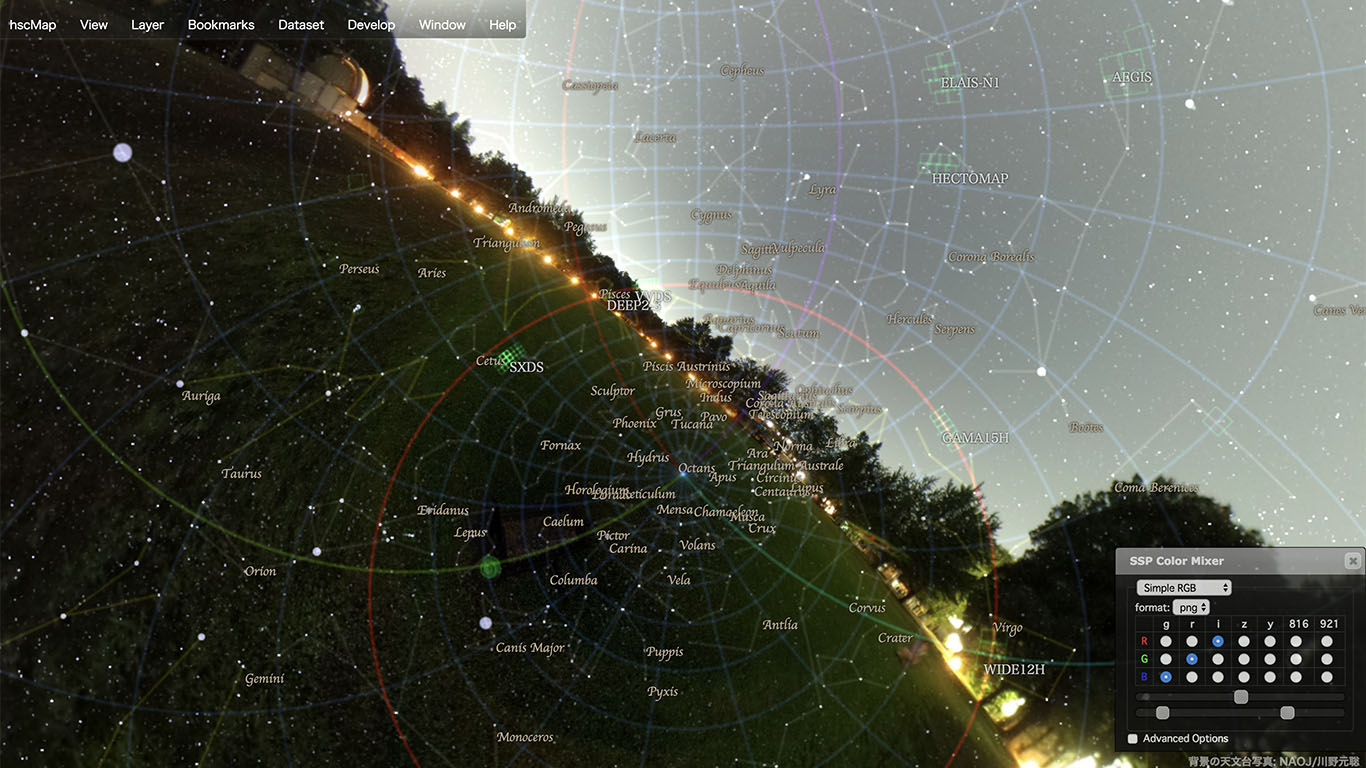
Fig. 2 Milky Way (left) and NAOJ Mitaka Campus (right) as the background. In the NAOJ Mitaka Campus photo, the dome of the 50-cm Telescope for Public Outreach is seen.
Bookmarks
- Add Bookmarks
- Edit Bookmarks
- Recommended Objects
- Gravitational Wave Source (GW170817): see the Fig. 3 below.
- SSP fields: go to an HSC-SSP field such as DEEP2-3 or VVDS
(When you select "patrol", you can cruise all of the fields.) - Import: import bookmarks
- Export: export bookmarks
- Show Bookmarks on the Sky
- Restore to Default
- Movement duration: Adjust the amount of time taken to cruise between objects or fields, in units of seconds.
-
When you select "patrol", you can tour all recommended objects.
See the "Recommended object bookmarks" page for individual recommended objects.
Gravitational Wave Source GW170817
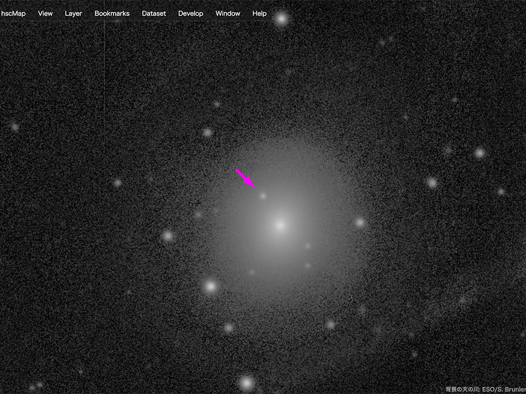
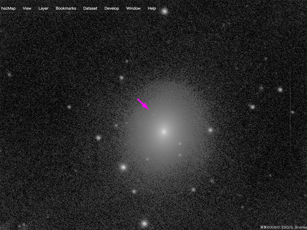
Fig. 3 Observation data taken with the Subaru Telescope of gravitational wave source GW170817 observed on August 17, 2017, with gravitational wave interferometers. (See the Press Release page of Subaru Telescope for more details.) When you select “Gravitational Wave Source (GW170817)” under “Bookmarks” on the menu bar, you can see the image from infrared observations. By holding down the shift key and pressing the “g” key (or by selecting “menu bar” > “Layer” > “Gravitational Wave Source” > “Next”, you can see the change in brightness of the gravitational wave source.
Dataset: observation fields to be displayed
- UDEEP: display the UltraDeep fields data
- DEEP:display the Deep fields data
- WIDE: display the Wide fields data
Develop
- Console
- Subaru Telescope: Please see Fig. 4 below.
- Telescope Lock: Please see Fig. 4 below.
- XYZ Axis
- View Frustum
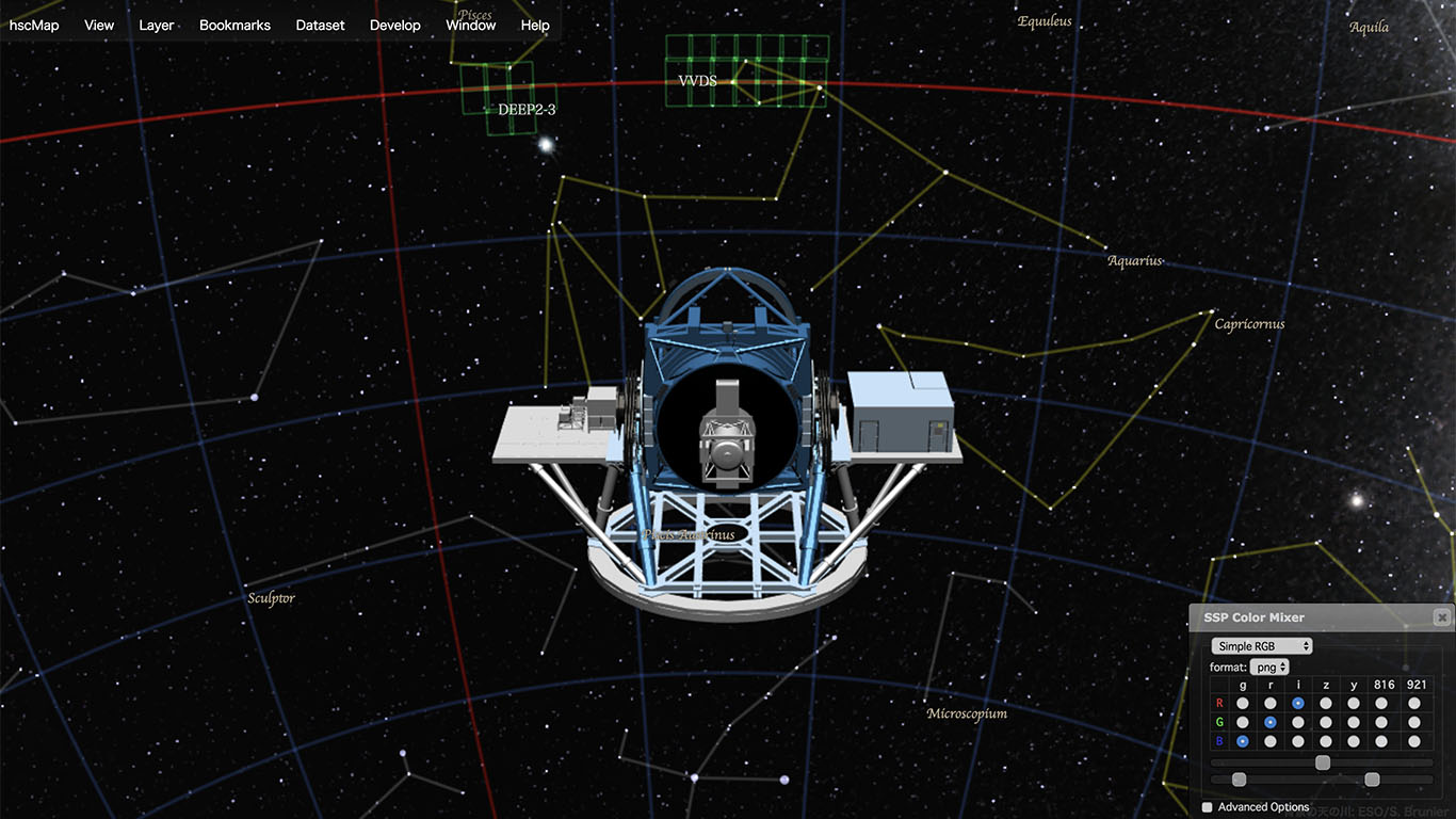
Fig. 4 When you select "Develop" > "Subaru Telescope" from the menu bar, an image of the Subaru Telescope is displayed. When you change the area of the sky, the telescope moves to point in the new direction. When you select "Telescope Lock", the telescope is fixed towards a certain direction in the sky.
Window
-
Select to open the relevant window. Please see the following chapter "Colors of objects in the HSC Viewer" for more about the "SSP Color Mixer" window.
"Colors" of objects in the HSC Viewer (Detail Information)
The human eye has three types of color receptors, known as cone cells. The three types of cones have good sensitivities in red, green, and blue light, respectively. The brain recognizes color by combining information (the ratio of stimulation) from the cones. When the red, green, and blue cones are activated with the same intensity, we perceive the color as white. On the other hand, when none of the cones are activated, we perceive the color as black. When the red and green colors are activated with the same intensity, we perceive the color as yellow. On a digital display, colors are shown by combining the intensities of red, green, and blue lights.
In astronomical observations, images taken at three different wavelengths, including wavelengths invisible to the human eye, are assigned the colors red, green, and blue and combined to create false-color composite images. The image at the longest wavelength is shown in red, the one at the intermediate wavelength is shown in green, and the one at the shortest wavelength is shown in blue. In the HSC-SSP survey, each layer (Wide, Deep, and UltraDeep) is observed in at least three wavelength bands. In the HSC Viewer by default, g (green) band images are shown in blue, r (red) band images are shown in green, and i (infrared) band images are shown in red. (You can change the color settings in the SSP Color Mixer window.)
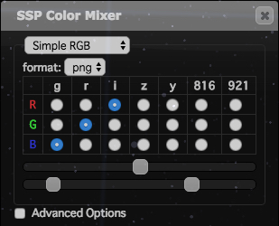
Fig. 5 The SSP Color Mixer window
You can change the color settings with this matrix. The band names (filter names) are listed from left to right, and display colors (Red, Green, and Blue) are listed from top to bottom. The bands are g(green, 4740 Å), r(red, 6170 Å), i(infrared, 7650 Å), z(infrared, 8890 Å), y(infrared, 9760 Å), NB816(infrared, 8180 Å), and NB921(infrared, 9210 Å). The first five are broad-band filters, and the last two are narrow-band filters. By default, the HSC Viewer shows g-band images in blue, r-band images in green, and i-band images in red. Please see the "Filters and limiting magnitudes" section in the "Large HSC dataset released to the public" page for more details.
Using the two bars under the matrix, you can adjust brightness and contrast (light-dark ratio). With the top bar, you can adjust the brightness of the entire display. When you move the knob to the right, the images become brighter (this function is similar to gamma correction). With the bottom bar, you can adjust the contrast. Pixels darker than the value of the left knob become black, and pixels brighter than the value of the right knob become white.